Self-attention

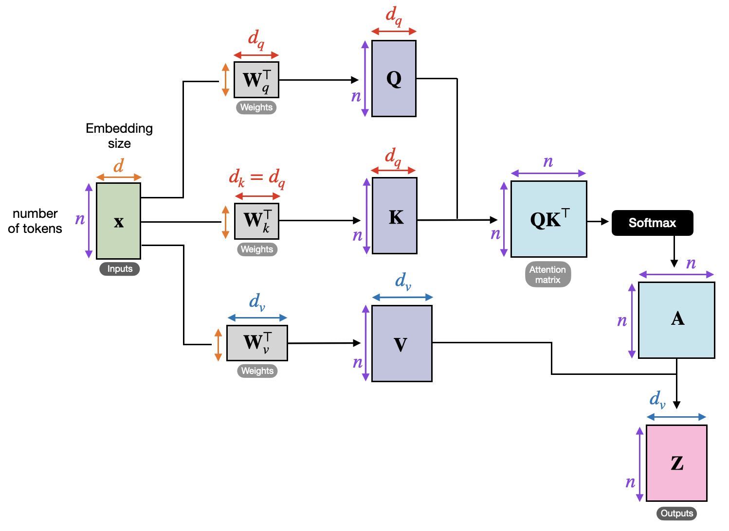
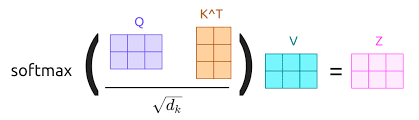
Self-attention is an attention mechanism in which each token in a sequence computes its representation by attending to all tokens in the same sequence, including itself. It enables the model to capture contextual relationships and dependencies regardless of their distance in the sequence. Mathematically, for an input sequence transformed into Query (Q), Key (K), and Value (V) matrices, self-attention is computed as:

where the similarity between queries and keys determines the attention weights, and these weights are used to compute a weighted sum of the value vectors. This allows each token to dynamically focus on the most relevant parts of the sequence to build richer contextualized representations.

How Attention Mechanism Works

You are given a sequence:

Past data → x₁, x₂, x₃, x₄, x₅, ..., xₜ
Goal → predict something at time t

Traditional thinking
Treat all past equally:

moving average
or sequential memory (RNN/LSTM)

But reality says:
Not all past is equally useful.

Human intuition
Imagine you’re analyzing markets today.
You don’t think:

“Let me average last 100 days”

Instead you think

“When did market behave like this before?”

Day	Market Condition	Should it matter?
1	calm uptrend	❌ low importance
2	calm uptrend	❌
3	slight drop	⚠️ medium
4	recovery	⚠️
5	volatility	✅ high
6	crash	🔥 very high

Your brain assigns weights

Day1 → 0.05
Day2 → 0.05
Day3 → 0.15
Day4 → 0.15
Day5 → 0.25
Day6 → 0.35

You are doing:

Compare present with past
Measure similarity
Assign importance
Combine information

Attention is:

NOT memory
NOT averaging

It is:

is a mechanism that learns where to look in the input by adaptive pattern matching over history

How Attention Decides What to Focus On

We now formalize attention as a mathematical operator.

1. Problem Setup

We are given a sequence:

X = x_{1}, x_{2}, \dots, x_{T}, x_{t} \in R^{d}

Goal: for each time step $t$ , compute a representation: $h_{t}$

$h_{t}$ should not depend only on $x_{t}$ , but should incorporate relevant information from other time steps.

So we aim for:

h_{t} = \sum_{τ = 1}^{T} α_{t, τ} \cdot x_{τ}

where:

$α_{t, τ}$ = importance of time $τ$ for time $t$

2. Learnable Projections

Instead of comparing raw inputs, we project them into three spaces:

q_{t} = W_{Q} x_{t}, k_{τ} = W_{K} x_{τ}, v_{τ} = W_{V} x_{τ}

where:

Q = [\begin{matrix} q_{1} \\ q_{2} \\ ⋮ \\ q_{T} \end{matrix}], K = [\begin{matrix} k_{1} \\ k_{2} \\ ⋮ \\ k_{T} \end{matrix}], V = [\begin{matrix} v_{1} \\ v_{2} \\ ⋮ \\ v_{T} \end{matrix}]

Here:

W_{Q}, W_{K}, W_{V} \in R^{d_{att} \times d}

Query $q_{t}$ : what the current timestep is looking for
Key $k_{τ}$ : representation of past timestep for comparison
Value $v_{τ}$ : information stored at timestep $τ$

Pasted image 20260407060325.png

3. Similarity Function

We compute similarity between time $t$ and $τ$ :

s_{t, τ} = q_{t}^{⊤} k_{τ}

q_{t}^{⊤} k_{τ} = | q_{t} | | k_{τ} | \cos (θ)

Large value → aligned → similar
Small value → unrelated

4. Scaling

We scale the dot product:

{\tilde{s}}_{t, τ} = \frac{q_{t}^{⊤} k_{τ}}{\sqrt{d_{att}}}

Without scaling:

variance of dot product grows with dimension
softmax becomes extremely sharp

5. Softmax Normalization

Convert scores into probabilities:

α_{t, τ} = \frac{\exp ({\tilde{s}}_{t, τ})}{\sum_{τ^{'}} \exp ({\tilde{s}}_{t, τ^{'}})}

α_{t, τ} \geq 0, \sum_{τ} α_{t, τ} = 1

So for each $t$ , $α_{t, τ}$ is a probability distribution over all timesteps.

6. Output Computation

Final representation:

h_{t} = \sum_{τ = 1}^{T} α_{t, τ} v_{τ}

h_{t} = \sum_{τ = 1}^{T} softmax (\frac{q_{t}^{⊤} k_{τ}}{\sqrt{d_{att}}}) v_{τ}

Matrix Form :

Attention (Q, K, V) = softmax (\frac{Q K^{⊤}}{\sqrt{d_{att}}}) V

Pasted image 20260419233656.png

At time $t$ :

h_{t} = \sum_{τ} α_{t, τ} v_{τ}

means:

construct today’s signal as a weighted combination of past regimes, where weights depend on similarity to current conditions

import numpy as np

def softmax(x):
    # subtract max for numerical stability
    x = x - np.max(x, axis=-1, keepdims=True)
    exp_x = np.exp(x)
    return exp_x / np.sum(exp_x, axis=-1, keepdims=True)

def attention(X, W_Q, W_K, W_V):
    """
    X: (T, d)
    W_Q, W_K, W_V: (d, d_attn)
    """

    # Step 1: Linear projections
    Q = X @ W_Q      # (T, d_attn)
    K = X @ W_K      # (T, d_attn)
    V = X @ W_V      # (T, d_attn)

    # Step 2: Similarity
    S = Q @ K.T      # (T, T)

    # Step 3: Scaling
    d_attn = Q.shape[1]
    S = S / np.sqrt(d_attn)

    # Step 4: Softmax
    A = softmax(S)   # (T, T)

    # Step 5: Output
    H = A @ V        # (T, d_attn)

    return H, A

Case Studies

Example

We are given a time series with 3 timesteps:

X = [\begin{matrix} 1 & 0 \\ 0 & 1 \\ 1 & 1 \end{matrix}]

We define projection matrices:

W_{Q} = [\begin{matrix} 1 & 0 \\ 1 & 1 \end{matrix}], W_{K} = [\begin{matrix} 1 & 1 \\ 0 & 1 \end{matrix}], W_{V} = [\begin{matrix} 1 & 0 \\ 0 & 2 \end{matrix}]

Attention Dimension: $d_{attn} = 2$
Compute the final attention output matrix

Step 1: Compute Q, K, V

Q = X W_{Q} = [\begin{matrix} 1 & 0 \\ 1 & 1 \\ 2 & 1 \end{matrix}]

K = X W_{K} = [\begin{matrix} 1 & 1 \\ 0 & 1 \\ 1 & 2 \end{matrix}]

V = X W_{V} = [\begin{matrix} 1 & 0 \\ 0 & 2 \\ 1 & 2 \end{matrix}]

Step 2: Compute Similarity Matrix

Transpose K

K^{⊤} = [\begin{matrix} 1 & 0 & 1 \\ 1 & 1 & 2 \end{matrix}]

Similarity Matrix,

S = Q K^{⊤} = [\begin{matrix} 1 & 0 \\ 1 & 1 \\ 2 & 1 \end{matrix}] [\begin{matrix} 1 & 0 & 1 \\ 1 & 1 & 2 \end{matrix}]

S_{1, 1} = 1 \cdot 1 + 0 \cdot 1 = 1

S_{1, 2} = 1 \cdot 0 + 0 \cdot 1 = 0

S_{1, 3} = 1 \cdot 1 + 0 \cdot 2 = 1

S_{2, 1} = 1 \cdot 1 + 1 \cdot 1 = 2

S_{2, 2} = 1 \cdot 0 + 1 \cdot 1 = 1

S_{2, 3} = 1 \cdot 1 + 1 \cdot 2 = 3

S_{3, 1} = 2 \cdot 1 + 1 \cdot 1 = 3

S_{3, 2} = 2 \cdot 0 + 1 \cdot 1 = 1

S_{3, 3} = 2 \cdot 1 + 1 \cdot 2 = 4

S = [\begin{matrix} 1 & 0 & 1 \\ 2 & 1 & 3 \\ 3 & 1 & 4 \end{matrix}]

Step 3: Scaling

S = [\begin{matrix} 1 & 0 & 1 \\ 2 & 1 & 3 \\ 3 & 1 & 4 \end{matrix}]

\tilde{S} = \frac{S}{\sqrt{d_{att}}} = \frac{S}{\sqrt{2}}

\tilde{S} \approx [\begin{matrix} 0.707 & 0 & 0.707 \\ 1.414 & 0.707 & 2.121 \\ 2.121 & 0.707 & 2.828 \end{matrix}]

Step 4: Softmax

Softmax formula applied to each element:

α_{i} = \frac{e^{x_{i}}}{\sum_{j} e^{x_{j}}}

Row 1

x = [0.707, 0, 0.707]

α_{1} = \frac{e^{0.707}}{e^{0.707} + e^{0} + e^{0.707}} = \frac{2.03}{2.03 + 1 + 2.03} = \frac{2.03}{5.06} \approx 0.401

α_{2} = \frac{e^{0}}{e^{0.707} + e^{0} + e^{0.707}} = \frac{1}{5.06} \approx 0.198

α_{3} = \frac{e^{0.707}}{e^{0.707} + e^{0} + e^{0.707}} = \frac{2.03}{5.06} \approx 0.401

Row 1 = [0.401, 0.198, 0.401]

Row 2

x = [1.414, 0.707, 2.121]

α_{1} = \frac{e^{1.414}}{e^{1.414} + e^{0.707} + e^{2.121}} = \frac{4.11}{4.11 + 2.03 + 8.34} = \frac{4.11}{14.48} \approx 0.284

α_{2} = \frac{e^{0.707}}{e^{1.414} + e^{0.707} + e^{2.121}} = \frac{2.03}{14.48} \approx 0.140

α_{3} = \frac{e^{2.121}}{e^{1.414} + e^{0.707} + e^{2.121}} = \frac{8.34}{14.48} \approx 0.576

Row 2 = [0.284, 0.140, 0.576]

Row 3

x = [2.121, 0.707, 2.828]

α_{1} = \frac{e^{2.121}}{e^{2.121} + e^{0.707} + e^{2.828}} = \frac{8.34}{8.34 + 2.03 + 16.93} = \frac{8.34}{27.30} \approx 0.305

α_{2} = \frac{e^{0.707}}{e^{2.121} + e^{0.707} + e^{2.828}} = \frac{2.03}{27.30} \approx 0.074

α_{3} = \frac{e^{2.828}}{e^{2.121} + e^{0.707} + e^{2.828}} = \frac{16.93}{27.30} \approx 0.620

Row 3 = [0.305, 0.074, 0.620]

Final Attention Matrix:

A = [\begin{matrix} 0.401 & 0.198 & 0.401 \\ 0.284 & 0.140 & 0.576 \\ 0.305 & 0.074 & 0.620 \end{matrix}]

Step 5: Compute Output

A = [\begin{matrix} 0.401 & 0.198 & 0.401 \\ 0.284 & 0.140 & 0.576 \\ 0.305 & 0.074 & 0.620 \end{matrix}]

V = [\begin{matrix} 1 & 0 \\ 0 & 2 \\ 1 & 2 \end{matrix}]

h_{t} = \sum_{τ = 1}^{T} A_{t, τ} \cdot v_{τ}

Row 1

h_{1} = 0.401 \cdot [1, 0] + 0.198 \cdot [0, 2] + 0.401 \cdot [1, 2]

= [0.401, 0] + [0, 0.396] + [0.401, 0.802]

= [0.802, 1.198]

Row 2

h_{2} = 0.284 \cdot [1, 0] + 0.140 \cdot [0, 2] + 0.576 \cdot [1, 2]

= [0.284, 0] + [0, 0.280] + [0.576, 1.152]

= [0.860, 1.432]

Row 3

h_{3} = 0.305 \cdot [1, 0] + 0.074 \cdot [0, 2] + 0.620 \cdot [1, 2]

= [0.305, 0] + [0, 0.148] + [0.620, 1.240]

= [0.925, 1.388]

Final Output

H = [\begin{matrix} 0.802 & 1.198 \\ 0.860 & 1.432 \\ 0.925 & 1.388 \end{matrix}]

Example

Market reacts to War News

We have 5 timesteps with price + news features:

x_{1} = [0.01, 0] (small return, no news)

x_{2} = [0.02, 0] (uptrend continues)

x_{3} = [- 0.05, 1] (WAR news + crash)

x_{4} = [- 0.02, 0] (aftershock)

x_{5} = [- 0.04, 1] (WAR escalation)

Feature meaning

First value = return
Second value = news signal (1 = war, 0 = none)

Value transformation

W_{V} = [\begin{matrix} 1 & 0 \\ 0 & 3 \end{matrix}]

So:

v_{t} = [return, 3 \times news]

Compute:

h_{5} = \sum_{τ = 1}^{5} α_{5, τ} v_{τ}

At time 5, model compares:

x_{5} = [- 0.04, 1]

Similarity reasoning

$x_{1}, x_{2}$ : no news → low similarity
$x_{3}$ : war + crash → HIGH similarity
$x_{4}$ : no news → moderate
$x_{5}$ : identical → highest

Approx attention weights

α_{5} \approx [0.05, 0.05, 0.35, 0.10, 0.45]

Compute values

v_{1} = [0.01, 0]

v_{2} = [0.02, 0]

v_{3} = [- 0.05, 3]

v_{4} = [- 0.02, 0]

v_{5} = [- 0.04, 3]

Output:

h_{5} = 0.05 v_{1} + 0.05 v_{2} + 0.35 v_{3} + 0.10 v_{4} + 0.45 v_{5} $ $ R e s u l t $ $ h_{5} \approx [- 0.038, 2.4]

Intuition

Model ignores calm periods
Focuses on past war events
Builds a “war-aware market state”

Key takeaway

h_{t} \neq x_{t}

h_{t} = context-aware regime representation

Pytorch Implementation

import torch
import torch.nn.functional as F

def attention_torch(X, W_Q, W_K, W_V):
    Q = X @ W_Q
    K = X @ W_K
    V = X @ W_V

    d_attn = Q.size(-1)

    S = Q @ K.transpose(-2, -1)
    S = S / torch.sqrt(torch.tensor(d_attn, dtype=torch.float32))

    A = F.softmax(S, dim=-1)
    H = A @ V

    return H, A